Symbolic execution. The first sign of using angr
1. Introduction
In today’s cybersecurity landscape, where threats are becoming increasingly sophisticated and complex, traditional vulnerability analysis methods often fall short. Finding and eliminating vulnerabilities is an ongoing process that requires constant improvement of tools and techniques. In this article, we’ll get acquainted with one of the most powerful and promising approaches—symbolic execution (symbolic execution)—and see how it can be effectively used with the angr.
Traditionally, security analysis relies on two main approaches: static and dynamic analysis. Static analysis, such as scanning code for known vulnerability patterns, has a number of limitations. It often produces many false positives, especially in complex projects, and cannot determine which parts of the code will actually execute for specific inputs. It also requires access to the application’s source code (white-box), which is not always possible during independent research.
From a reverse-engineering perspective (black/gray-box testing), analysts use disassembly and decompilation followed by manual analysis. In this case, a full application review requires a huge amount of time and expertise, and is often practically impossible due to the size of modern programs. And even with this approach, there is no guarantee of results.
Dynamic analysis, on the other hand, involves running a program with concrete inputs and monitoring its behavior. This approach can uncover vulnerabilities that only manifest at runtime, but it requires careful input selection to achieve sufficient code coverage. Finding inputs that trigger “deep” or rarely used code paths can be extremely difficult, especially for large and complex programs. In addition, dynamic analysis does not guarantee that all possible execution paths will be explored. If the inputs never cause the vulnerable code to execute, it will remain unnoticed. Moreover, vulnerable states are often associated with boundary values of variables; therefore, reaching a vulnerable part of a program does not always mean the vulnerability will be detected.
Let’s look at a simple example:
#include <stdio.h>

int main(int argc, char *argv[]){
    char name[10];
    scanf("%s", name); // buffer overflow
    printf("Hello, %s\n", name);
    return 0;
}
A classic buffer overflow: a program accepts a string as input and copies it into a fixed-size buffer. A static analyzer may flag this vulnerability, but it cannot derive the exact inputs needed to exploit it. Dynamic analysis would require providing a string longer than the buffer to trigger an overflow. If we provide a shorter string, the vulnerability will go unnoticed.
2. Symbolic execution.
Symbolic execution offers an elegant solution to these problems. Instead of analyzing a program with concrete inputs, we can use symbolic variables such as “x” that represent any possible value. As we traverse the program’s execution branches, we build a path predicate—a logical expression describing constraints on the inputs. In this way, symbolic execution can potentially achieve very high path coverage that other methods cannot, although for very large programs full coverage may be limited by the “state explosion” problem, where the number of possible paths grows exponentially, making exhaustive analysis computationally expensive.
Let’s make the previous example a bit more complex: now the program doesn’t just ask for your name and greet you—it computes a coefficient based on your balance and age, and under certain conditions offers to save your data, where the buffer overflow vulnerability resides.
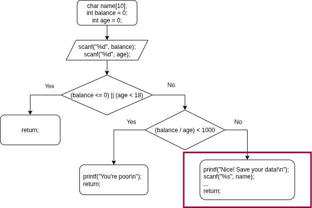
The symbolic execution engine will split this program into three paths, and for each of them it will build the corresponding constraints (predicates). This lets us find conditions that “activate” specific parts of the code, even if they are rarely executed.
We can now think of the program as an “execution tree,” where each node corresponds to a specific symbolic state, and the branches represent different paths caused by conditional jumps. To fully understand how this works, let’s break down the key concepts behind this approach: the SMT solver, symbolic variables, and the symbolic state.
Satisfiability Modulo Theories (SMT, the satisfiability problem for formulas modulo theories) is the problem of deciding logical formulas while taking into account the theories they are built on—for example, theories of integers and real numbers, lists, bit-vectors, and so on.
In our case, we will use the theory of bit-vectors. Working with them is largely similar to operations on integers, but with one key difference: the stored value is limited by the vector size. If the result of an operation does not fit into the allotted number of bits, the most significant part that exceeds the vector bounds is discarded. Mathematically, this means that all arithmetic operations are performed modulo 2^N, where N is the vector size in bits.
For example, for a 1-byte variable (N=8), computations are performed modulo 2^8 = 256. Its range of values is from 0 to 255. If you add 1 to the maximum value 255, the result is (255 + 1) mod 256 = 0. This principle works for vectors of any size, whether it’s a standard word (N=16, modulus 65536) or a non-standard 3-bit vector (N=3, modulus 8).
To solve practical problems, we use SMT solvers. The best-known one is Z3, developed by the Microsoft Research team; it is the one used to solve logical expressions in the angr framework.
A symbolic variable is a variable that denotes an unknown value, yet can still be used in computations. In a sense, it is closer to the mathematical notion of a “variable” than to a programming variable.
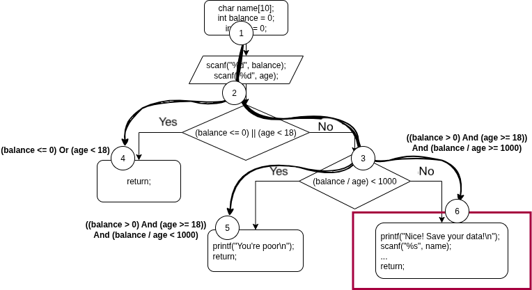
During symbolic execution, symbolic expressions are built from these variables. For example, to reach node 3 (Fig. 2), balance must be > 0 and age must be >= 18; then, to reach node 6, we add the condition that the balance-to-age ratio must be at least 1000.
The resulting expression is passed to the SMT solver, which can answer questions such as: is this code region reachable at all? Can we find concrete values for the variables to enter this branch?
The result can be SAT and UNSAT:
SAT (Satisfable): means that a solution exists and can be computed
UNSAT (Unsatisfable): means: “no, there is no value that satisfies all conditions at once.” In other words, this execution path is unreachable.
Symbolic program state is the collection of values of variables, registers, and memory cells while symbolically executing a program. The main difference from a “traditional” state is that, in addition to concrete values, registers and memory cells may contain logical expressions.
3. Angr
Now that we’ve covered the theoretical foundations of symbolic execution, it’s time to look at the tool that brings these ideas to life: angr is a powerful and flexible Python framework for analyzing binary files. It provides a rich set of tools for automating reverse-engineering tasks and vulnerability research, and at its core lies a symbolic execution engine.
Angr lets us programmatically explore binaries without running them in the traditional sense. It abstracts away complex CPU and OS details, allowing us to focus on program logic.
3.1. Installing angr
There are several ways to install angr on your system; they are described here. The simplest is installing via pip.
# pip install angr
You can verify a successful installation right in the Python command line:
>>> import angr
>>> angr.__version__
'9.2.100'
3.2. Key components of angr
Once the environment is prepared, we can move on to practice. Working with angr revolves around several core objects that correspond to the concepts we discussed earlier.
The first key component in angr is Project, which is the main object throughout the analysis. A Project object is created by loading a binary. When loading, angr analyzes the file, determines its architecture (x86, ARM, etc.), format (ELF, PE), entry point, and maps the binary code into a virtual address space.
import angr
# Load the file into the project
project = angr.Project('./sample1')
The next key component is the state (State). In angr, a state (a node in our “execution tree”), or SimState is a complete snapshot of the program state at one particular moment in time. This includes everything: register values, memory contents, and even filesystem state (for example, data read from standard input).
Recall that the key difference of SimState from a traditional program state is that it can operate on symbolic variables. To start the analysis, we need to create an initial state.
The simplest way to create an initial state is to use the program’s entry point.
initial_state = project.factory.entry_state()
If you need to analyze a specific function, or start not from the entry point, it’s better to use another method:
initial_state = project.factory.call_state(address=0x1189)
# Where 0x1189 is the function address
Now that we have an initial state, we need a way to explore how this state will change as the program executes. For this, we use the Simulation Manager. It takes the initial state (or multiple states) and starts stepping the program. When angr encounters a conditional jump (for example, if-else), the Simulation Manager “forks” the current state into two new ones: one for the if branch and one for the else branch, adding the corresponding constraints to each.
It manages all active execution paths, tracking them in dedicated containers (stashes):
- active - states that are ready for further exploration.
- deadended - states that can no longer execute for various reasons (end of code, error, etc.).
- found - states that have reached the target address.
- avoided - states that have reached an address we want to avoid (if we realize execution went the wrong way).
- and others, for more complex scenarios.
# Create a Simulation Manager with the initial state
simgr = project.factory.simulation_manager(initial_state)
These objects are generally enough to start exploring the target program, but we’re still missing the most important component of symbolic execution—symbolic variables.
3.3 Claripy
To work with symbolic variables in angr, the module claripy is used; it ties together “under the hood” several technologies, including the Z3 SMT solver.
# Import the module
import claripy
# Declare symbolic variables
a = claripy.BVV(3, 32)       # Symbolic constant 3, 32 bits wide
b = claripy.BVS('var_b', 32) # Symbolic variable var_b, 32 bits wide
s = claripy.Solver()         # Main object — the SMT solver
s.add(b > a)                 # Add a logical constraint to the solver
print(s.eval(b, 1)[0])       # Find a value for the variable
You may have noticed a small but fundamental difference between the variables a and b. Variable a is a BVV (Bit-Vector Value), while variable b is a BVS (Bit-Vector Symbolic Variable).
- BVV - a constant; it represents a known value of a fixed size.
- BVS - a symbolic variable.
They are critically important for the SMT solver: BVS is the unknown we’re solving for, and BVV is part of the constraints.
Since we already have the full list of logical constraints (Figure 2) that define the flow toward the desired code branch, namely:
((balance > 0) And (age >= 18)) And (balance / age >= 1000)
We can solve this ourselves using claripy:
# Create the solver
s = claripy.Solver()
# Declare variables
balance = claripy.BVS("balance", 31)
age = claripy.BVS("age", 31)
# Add constraints
s.add(balance > 0)
s.add(age >= 18)
s.add(balance/age >= 1000)
# Compute the result
print(f"balance: {s.eval(balance,1)[0]}")
print(f"age: {s.eval(age,1)[0]}")
Each time you run this script, you’ll get different values that satisfy the constraints. Note that the variable size is 31 bits, while an integer is 32 bits—why? This is because an int is a signed type, and the most significant bit encodes the sign: 0 for a positive number, 1 for a negative one. The value itself occupies the lower 31 bits.
1. balance: 1149100004
   age: 25
2. balance: 1878988608
   age: 112
3. balance: 999157188
   age: 132115
All of these values satisfy the constraints and drive execution toward the vulnerable code. We can also find the minimum and maximum values of the target variables using the methods min() and max() respectively.
min: balance: 18000
     age: 18
max: balance: 2147483647
     age: 2147483
3.4 Final stage
Now we can move on to writing the script to analyze the program from our example.
import angr
import claripy # Needed to declare symbolic variables

# Create the project
project = angr.Project("./sample1")
Before creating the initial state, we need to declare the symbolic variables representing the input. Since all data in our program is read from standard input (stdin) we will create a single symbolic variable for the entire input.
# Declare symbolic stdin
symbolic_stdin = claripy.BVS("stdin", 10 * 8) # size: 10 bytes
# Create the initial state at the entry point, passing our symbolic data as stdin
initial_state = project.factory.entry_state(stdin=symbolic_stdin)
# Create the Simulation Manager
simgr = project.factory.simulation_manager(initial_state)
To search for a path to a specific address, Simulation Manager provides the method explore(), where you use the “find” argument to specify the target address.
For clarity, the source code of the program being analyzed is shown below.
#include <stdio.h>

int main(){
    char name[10];
    int balance = 0;
    int age = 0;

    scanf("%d", &balance);
    scanf("%d", &age);

    if ((balance <= 0) || (age < 18)){
        return 1;
    }
    else if ((balance / age) < 1000)
    {
        printf("You're poor\n");
        return 1;
    }
    printf("Nice! Save your data!\n");
    scanf("%s", name);
    return 0;
}
As mentioned earlier, the buffer overflow vulnerability arises because a string is written into a buffer without checking its size. But to exploit it, you need to reach the part of the code where this write happens. Below is the control-flow graph of the analyzed function in IDA Pro (Figure 3). For symbolic analysis we don’t care about the entire program; we only need to find the vulnerable block and determine its address (Figure 4):
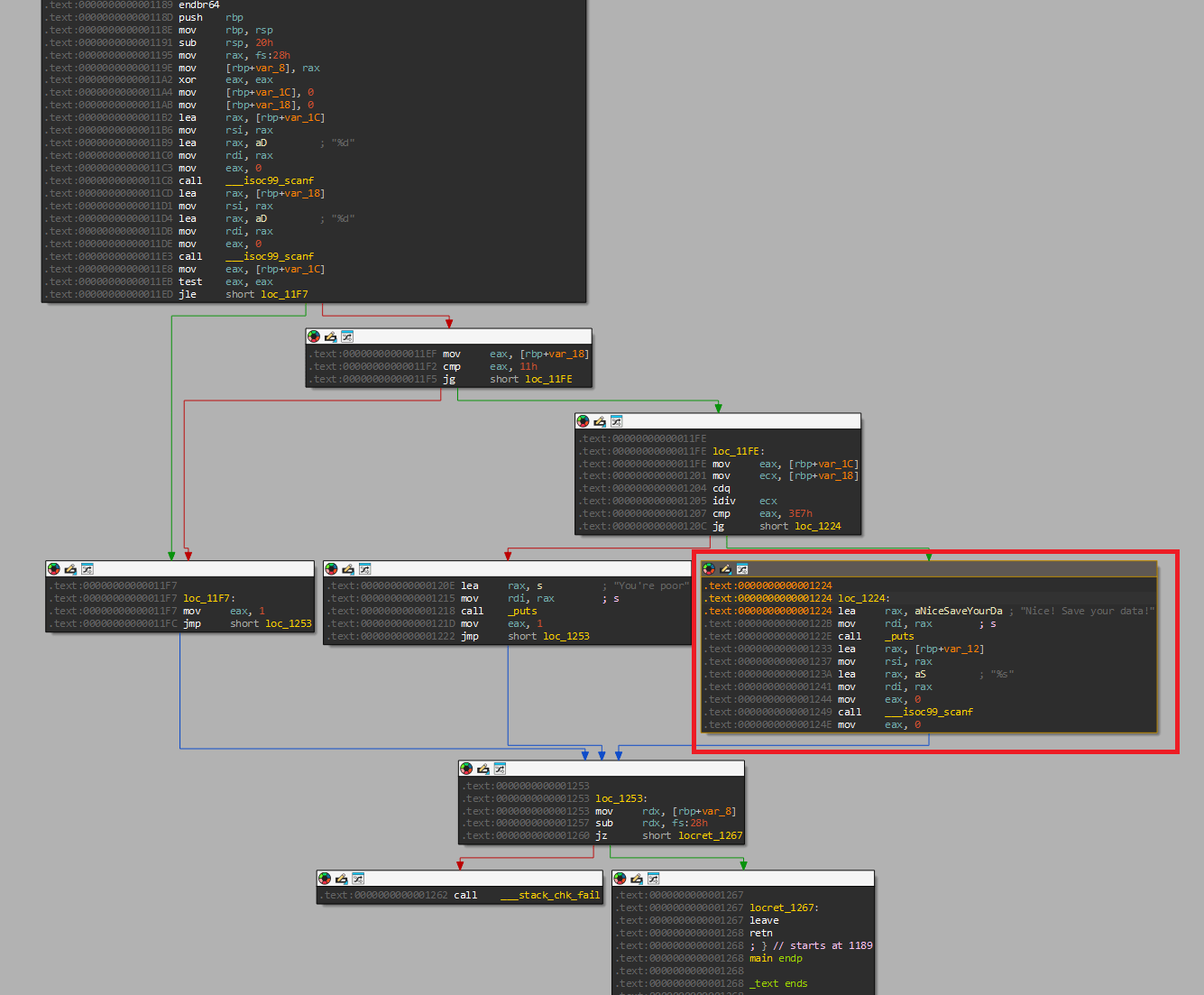
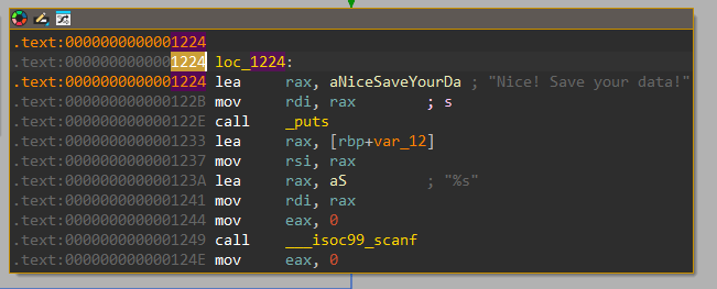
In our case, the target address is 0x1224, but remember that this is an address relative to the start of the file. When loaded into memory, it will be mapped at some base address. You can obtain this address at runtime and simply add it to the target offset.
# Determine the base address
base_addr = project.loader.main_object.mapped_base
# Compute the address of the vulnerable block
find_addr = 0x1224 + base_addr
# Start the search
simgr.explore(find=find_addr)
Angr will stop on its own as soon as it finds the first path that satisfies the constraints, or once all paths have completed execution. If a desired path is found, the corresponding symbolic state is placed into the found stash.
if simgr.found:
    # Get the first found path/state.
    found_state = simgr.found[0]
Now we pass the symbolic variable to the SMT solver and ask it to find a concrete solution for the symbolic stdin that satisfies all constraints collected along this path.
# Evaluate the symbolic stdin. cast_to=bytes converts the result to a byte string.
solution_stdin = found_state.solver.eval(symbolic_stdin, cast_to=bytes)
Final script:
import angr
import claripy # Needed to declare symbolic variables

# Create the project
project = angr.Project("./sample1")

# Declare symbolic stdin
symbolic_stdin = claripy.BVS("stdin", 10 * 8) # size: 10 bytes
# Create the initial state at the entry point, passing our symbolic data as stdin
initial_state = project.factory.entry_state(stdin=symbolic_stdin)
# Create the Simulation Manager
simgr = project.factory.simulation_manager(initial_state)
# Determine the base address
base_addr = project.loader.main_object.mapped_base
# Compute the address of the vulnerable block
find_addr = 0x1224 + base_addr
# Start the search
simgr.explore(find=find_addr)

if simgr.found:
    # Get the first found path/state.
    found_state = simgr.found[0]
    # Evaluate the symbolic stdin. cast_to=bytes converts the result to a byte string.
    solution_stdin = found_state.solver.eval(symbolic_stdin,
                                             cast_to=bytes)
    print(solution_stdin)
As a result of running the script, we got the answer “8392084+20”. The “+” symbol doesn’t matter here: the program will read two integers in sequence—8392084 and 20—which satisfies the conditions and leads us to the vulnerable part of the code.
4. Conclusion
In this article, we went from the theoretical foundations of symbolic execution to its practical application with the angr framework. We saw how this approach can automatically find inputs that steer a program along a specific execution path, thereby effectively overcoming the key limitations of traditional static and dynamic analysis.
The example we discussed is only a starting point. Symbolic execution is indispensable for automatic exploit generation (AEG), reverse engineering proprietary protocols, and verifying program correctness.
Of course, symbolic execution has its limitations. The main issue is “state explosion.” In addition, accurately modeling interactions with the outside world (the system, network) remains challenging.
Despite these difficulties, symbolic execution remains one of the most advanced and effective tools in the arsenal of a security researcher and reverse engineer. Learning angr enables you to automate complex analysis tasks that previously required many hours of manual work.